Climate risk modeling is no longer the exclusive domain of ESG teams. As climate change begins to impact core financial drivers like utility and insurance costs, investment analysts, corporate strategists, and financial planners alike are recognizing the importance of integrating climate impact into financial decision-making.
Yet, many still lack the tools and frameworks to do this effectively. To help close this gap, AlphaGeo is launching a new series — Climate Finance 101 — to demystify how climate risks translate into financial impact. In this first installment, we explore how climate change impacts utility demand and costs, and how organizations can integrate these insights into financial modelling and decision-making.
🌡️ How Climate Change Affects Utility Demand
The effect of climate change on energy consumption is regionally variable and climate specific. Accurately modeling this requires understanding the local balance between heating and cooling demand. Where temperatures are rising, we expect:
- Cooling demand to increase in warmer seasons
- Heating demand to decrease in colder seasons
While some colder regions may benefit from lower winter energy use, these savings are often outweighed by increased cooling needs during hotter summers — resulting in a net rise in energy consumption in many locations worldwide.
🧮 Measuring and Modeling Impact
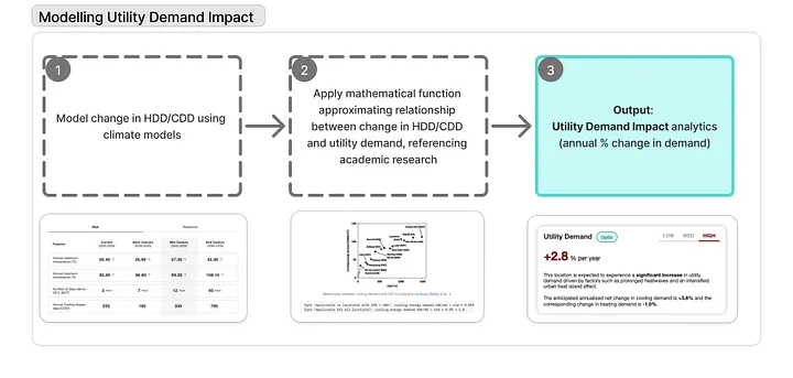
AlphaGeo models the impact of climate change on utility demand using a combination of Degree Day forecasting and energy demand functions.
We begin by forecasting changes in Cooling Degree Days (CDD) and Heating Degree Days (HDD) — proxies of building energy consumption. Despite their name, Degree Days are not a measure of time but rather of how far outside air temperatures deviate from a baseline considered thermally comfortable (typically 18°C / 65°F). The more extreme the outside temperature relative to the baseline, the higher number of degree days, with:
- Cooling Degree Days (CDD) indicating demand for cooling (in warmer weather)
- Heating Degree Days (HDD) indicating demand for heating (in colder weather)
We use climate models to understand the change in CDD or HDD under various climate scenarios. We then apply empirically derived functions from academic literature to estimate the corresponding change in heating and cooling demand.
Finally, we compare the net heating/cooling demand for a future year (e.g., for 2050) with a baseline year (currently 2025) to estimate the annual change in heating and cooling demand.
(Note: For more technical detail, visit our methodology documentation here.)
🌍 Results: Global Patterns in Utility Demand
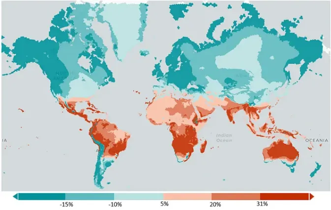
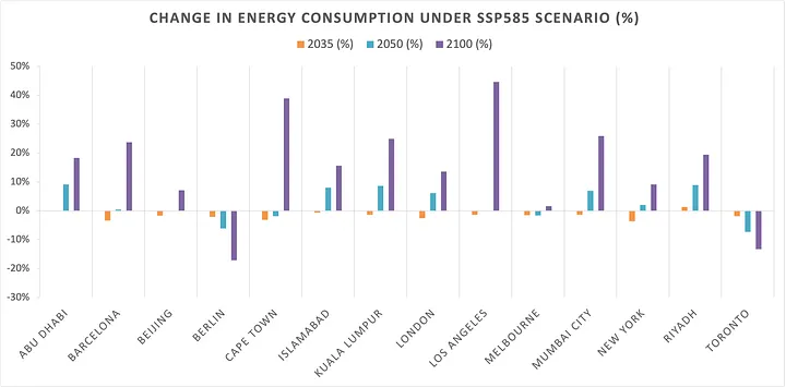
Using this methodology, our research finds that while global energy consumption on the whole is expected to rise, tropical regions and parts of the Southern Hemisphere will be disproportionately affected (Map 1). Conversely, some cities in cooler climates may see energy savings. For example, cities such as Toronto and London are expected to experience reduced energy consumption, while Riyadh and Kuala Lumpur will likely face significant increases (Chart 2).
Trends, moreover, are expected to evolve over time. By 2100, cities such as Cape Town, Barcelona, and Beijing show a shift from decreased to increased energy use, underscoring the importance of long-term scenario planning (Chart 2).
💡 Why This Matters
Understanding changes in utility demand has meaningful implications for a range of stakeholders:
- 📊 Valuation & investment analysts: Use climate-adjusted demand assumptions for more robust valuation or returns modelling, or perform sensitivity analyses under different climate scenarios.
- 📉 Financial planners & analysts: Revise operating cost forecasts to reflect shifts in utility expenses.
- 🏛️ Policy planners: Plan energy infrastructure and regulatory frameworks with changing demand in mind.
🔍 Use Case: Climate-adjusted Sensitivity Analysis
Let’s consider a simplified example of a commercial building, which is experiences a baseline energy cost increase of 2%.
Using AlphaGeo’s Financial Impact Analytics toolkit, we further estimate climate-driven changes in utility demand under the following scenarios:
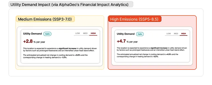
This gives us the following set of assumptions on the annual change in energy costs:
- Baseline: 2% (inflation)
- Medium Emissions Scenario: 2% (inflation) + 2.8% (climate impact) = 4.8%
- High Emissions Scenario: 2% + 4.7% = 6.7%
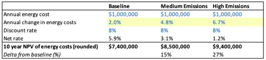
Putting it all together, we see that a High Emissions scenario could result in an additional 30% in energy costs compared to the baseline, assuming a 8% discount rate over 10 years (Table 1).
The above is, of course, a highly simplified example. In a real-world context, these assumptions can used by investment analysts to conduct sensitivity analyses across climate scenarios, or integrated directly as cost inputs into internal investment or financial models.
🔚 Conclusion
As climate change accelerates, understanding its financial implications — including on energy consumption — is no longer optional. AlphaGeo’s Financial Impact Analytics toolkit was developed precisely to help our clients integrate scientifically-grounded climate data into real-world financial planning. What was once the responsibility of sustainability teams can now become a core competency across investment teams and business units.
📬 Learn More
Insights and Research: Follow us today on LinkedIn or Medium to receive updates on our Climate Finance 101 series, alongside other insights.
Financial Impact Analytics: Learn more about how our Financial Impact Analytics suite helps translate climate risk into financial impact here.
Other Solutions: Learn more about us at alphageo.ai, or reach out at info@alphageo.ai to schedule a call.